4. Retriever Module
4.1. Launching the retriever
Launching the retriever as a stand-alone program:
Follow the steps to install PyMoDAQ Femto (see Installation section)
Open a shell (for instance, Anaconda Prompt) with the correct conda environment activated
Type
retriever
Launching the retriever from a PyMoDAQ Dashboard:
Load your dashboard
In the top bar menu, go to Extensions/FemtoRetriever
4.2. Overview of the retrieval procedure
The interface of the retriever is shown below:
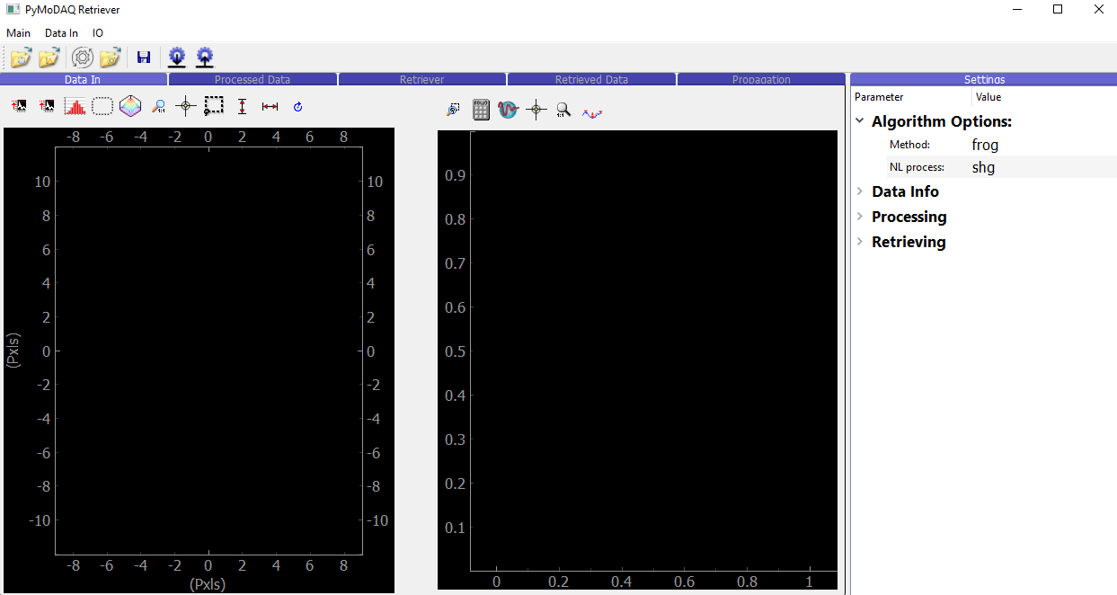
Fig. 4.1 Interface of the retriever module of PyMoDAQ-Femto (before loading any data).
The blue tabs follow the general retrieval procedure:
Data In: Data is imported, displayed, and regions of interest can be selected
Processed Data: The non-linear trace is pre-processed and interpolated on a user-defined grid
Retriever: An iterative algorithm tries to reproduce the measured trace. Each iteration is displayed during the retrieval
Retrieved Data: The best solution is displayed and compared to the measurement
Propagation: Arbitrary amounts of material (air, glass, etc.) can be added to the pulse to simulate how the pulse will look like after propagation.
4.3. Loading data
The retriever handles both data simulated by the Simulator Module and experimental data.
We strongly recommend that you experiment with the retriever on simulated data before attempting to retrieve experimental data.
4.3.1. Loading simulated data generated by the simulator module
Click the wheel  icon in the top menu to launch the simulator. If you are not familiar with its behavior, check out the documentation here: Simulator Module.
Set up the pulse and the trace as you like. Here we will use the default values for everything, except the method: instead of the default SHG frog, we will use PG frog. This should generate the same trace as the PyMoDAQ-Femto logo that you see at the top left of this page!
Then, go back to the retriever and click the  icon. Both the trace and the fundamental spectrum should now be displayed as shown below.
The data viewers use the PyMoDAQ viewers, which have many functionalities available: lineouts, regions of interest, cursors, rescaling of axes, colormap changes, etc.
icon. Both the trace and the fundamental spectrum should now be displayed as shown below.
The data viewers use the PyMoDAQ viewers, which have many functionalities available: lineouts, regions of interest, cursors, rescaling of axes, colormap changes, etc.
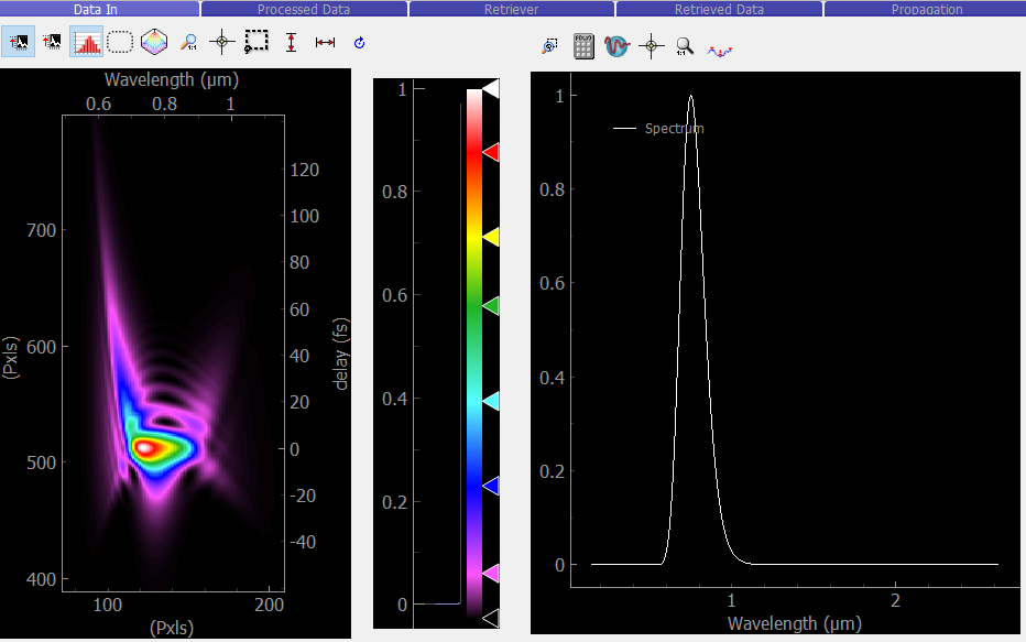
Fig. 4.2 Retriever with data loaded from simulator.
4.3.2. Loading experimental data
4.3.2.1. Data measured using PyMoDAQ
If your data was measured using PyMoDAQ Scan function, then we have good news for you: they already have the proper formatting and will seamlessly load into PyMoDAQ-Femto!
To load the trace, click the  Load Experimental Trace icon, and navigate to your .h5 file. It will open your file in H5Browser. Select the Data node corresponding to the trace and double-click it.
Lineouts of the trace will be displayed as shown below. Then, click OK to load the trace.
Load Experimental Trace icon, and navigate to your .h5 file. It will open your file in H5Browser. Select the Data node corresponding to the trace and double-click it.
Lineouts of the trace will be displayed as shown below. Then, click OK to load the trace.
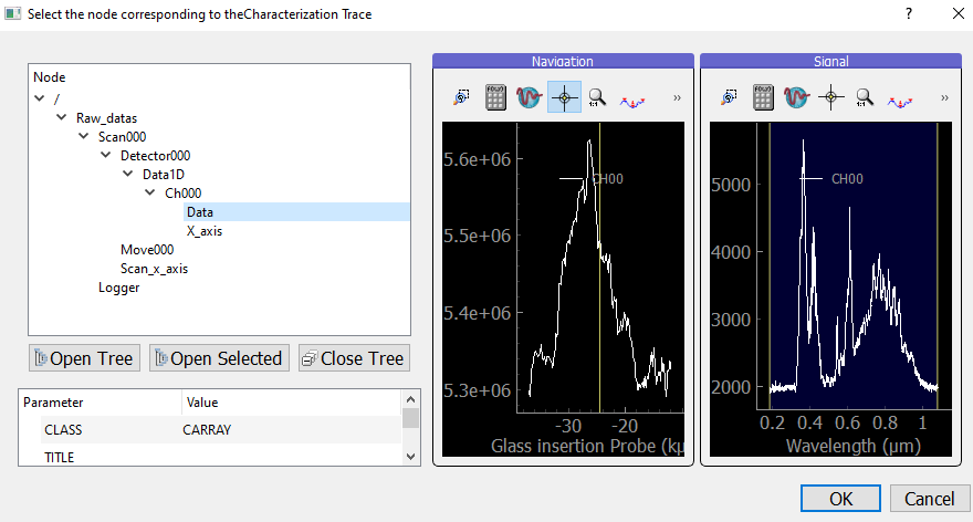
Fig. 4.3 Loading the trace node from a .h5 file.
To load the fundamental spectrum, click the  Load Experimental Spectrum icon and repeat the same steps to load the spectrum.
4.3.2.2. Converting raw data to be used in the retriever
If the non-linear trace was measured using another acquisition program than PyMoDAQ, we are slightly disappointed but will nonetheless explain how to convert it the proper format before being loaded into the retriever. PyMoDAQ-Femto uses a binary format known as hdf5, as described in the PyMoDAQ documentation.
We provide an example script to convert raw data, located inside the PyMoDAQ-Femto module, under pymodaq_femto/utils/convert_to_pymodaq_compatible.py.
If you are using conda with a dedicated environment as suggested in the Installation section, this folder will be located inside the site-packages folder, for instance in Windows something like:
C:/Miniconda/envs/your_environment_name/Lib/site-packages/pymodaq_femto
This /utils folder is also easily accessible on GitHub.
If it is not already the case, raw data should be converted to numpy arrays. 5 arrays are needed:
The 2D trace [N x M numpy array]
An array corresponding to the parameter axis (delay in Frog, glass insertion in Dscan, etc.) in physical units [N x 1 numpy array]
An array with the wavelength axis of the trace [M x 1 numpy array]
The fundamental spectrum (spectrum of light before non-linear conversion) [P x 1 numpy array]
The wavelength axis of the fundamental spectrum [P x 1 numpy array]
Note
The retriever has an option to rescale any input array, so parameter or wavelength axes can be saved in any units. That being said, it is usually easier to save all data in standard units everytime (meters for wavelengths and insertions, seconds for delays, etc.).
The fundamental spectrum doesn’t need to be on the same wavelength axis as the 2D trace, they will get interpolated on a common axis during retrieval. The role of the fundamental is to compare retrieved spectrum with measured one (a good measure of the quality of retriever), and can also be used as an initial guess for the algorithm. But if you don’t have one for every trace, just use any spectrum you have and the algorithm will still work.
Once the 5 numpy arrays are loaded, you can use the utility functions of pymodaq_femto/utils/convert_to_pymodaq_compatible.py to create a new .h5 file
and add all data to it, with the proper structure.
Example:
One raw DScan measurement (not measured with PyMoDAQ) is provided in pymodaq_femto/utils/raw_scans/example_measured_dscan_to_convert.h5. The 5 numpy arrays are stored in there.
The example file pymodaq_femto/utils/convert_to_pymodaq_compatible.py converts this file into a PyMoDAQ-Femto-compatible h5 file.
The file is loaded, and the 5 numpy arrays are extracted:
parameter_axis = measured_dscan.axes[0]
spectrum_trace_axis = measured_dscan.axes[1]
spectrum_fundamental_intensity = raw_spectrum.intensity
spectrum_fundamental_axis_wavelength = raw_spectrum.wl
trace_data = measured_dscan.data
Since this example is a DScan trace, the parameter is the insertion of glass in the beam, expressed in meters. For a FROG trace, the parameter would be the time delay between two pulses, in seconds.
Then the script initializes a new .h5 file and gives it the correct structure:
saver = PyMoDAQFemtoCustomSaver()

# Open file and create scan node
saver.init_file(addhoc_file_path=str(pathToSave.joinpath(fileName)), update_h5=True)
scannode = saver.add_scan_group()
scannode.set_attr('scan_type', "Scan1D")
And finally we add data to it, using the convenience functions:
# Add all data
saver.add_exp_parameter(scannode, parameter_axis, label='Insertion', units='m')
saver.add_exp_trace(scannode, trace_data, spectrum_trace_axis)
saver.add_exp_fundamental(scannode, spectrum_fundamental_intensity, spectrum_fundamental_axis_wavelength)
saver.close_file()
The script should save a converted file into pymodaq_femto/utils/converted_scans/, that can be directly loaded into the retriever.
4.4. Pre-processing data
4.4.1. Method definition and data rescaling
Once the data is loaded, the parameter tree on the right of the interface gets populated with several values. When working with data generated by the simulator module, everything will be set correctly. However, it won’t be the case for experimental data, and some parameters are important to set correctly:
Algorithm Options:
Method:
(type: list)The type of measurement (FROG, DSCAN, etc.). See Available methods for a full list of available methods. This must match the method experimentally!NL process:
(type: list)The non-linear process to use (second harmonic generation, third harmonic generation, etc.). This must match the method experimentally!
Data Info
Trace Info
Wavelength Scaling
(type: float)Scaling to convert the wavelength axis of the experimental trace into meters.Parameter Scaling
(type: float)Scaling to convert the parameter axis of the experimental trace into correct unit (meters for DScan, seconds for FROG, etc).
Spectrum Info
Wavelength Scaling
(type: float)Scaling to convert the wavelength axis of the experimental fundamental spectrum into meters.
The scalings allows handling of data taken in any units. They also allow flexibility, for instance, the axis of the measured trace might be the position of a motor. You can use these scalings to convert it to delay, glass insertion, etc.
Note
After using the retriever on a daily basis in our labs, we find that in the majority of cases, weird behaviors come from incorrect scaling parameters, or having the wrong Method select (Frog instead of Dscan)! If the retrieved trace look like rubbish, the first thing to do is to look at the measured trace and verify that its axes are correct!
4.4.2. Grid settings
Then, you must choose the grid on which the pulse will be computed. The definition is made using both temporal or spectral property, depending on which is more convenient.
Grid settings:
lambda0 (nm):
(type: float)The central wavelength of the grid in the spectral domain, in nanometres. By default, it uses the center of the measured fundamental spectrum.Npoints:
(type: list)Number of points of the grid (both in spectral and temporal domain). More points will require more type to retrieve the pulse, but increases the spectral resolution and the width of grid in the temporal domain.Time resolution (fs):
(type: float)The time between two points of the grid in the temporal domain.
4.4.3. Background and region of interest
Trace limits:
If you tick this box, a rectangle will appear on the measured trace. It allows to select the region of interest that will be used for the retrieval. You can either move and resize the rectangle, as shown below, or use the x0, y0, width, height parameters in the parameter tree.
Substract trace background:
If you tick this box, two vertical lines will appear on the measured trace. The data between these lines will be averages and used as the background for the trace. You can either move the two lines, or use the wl0, wl1 parameters in the parameter tree. The background region must be inside the region of interest.
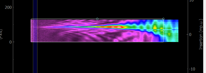
Fig. 4.4 Selecting the region of interest (rectangle) and background region (vertical lines) of a measured trace.
Substract spectrum background:
Same as the trace, but for the fundamental spectrum.
Once all this is set, press the button Process Both to proceed. This will take you to the next tab (Processed Data) which shows you data ready to be retrieved. The pulse displayed in time and frequency on the right is the Fourier Transform-limited pulse obtained from your fundamental spectrum, interpolated on the defined grid. Verify that the trace looks good, and that your temporal and spectral grids are adequate and proceed to the retrieval.
4.5. Running the retrieval algorithm
Here there are a few parameters to choose from. We recommend sticking with default ones for the most part, but feel free to experiment with everything
Retrieving
Algo type:
(type: list)Retrieval algorithm to use. Recommended: copra. These are implemented in pypret, the whole list of available algorithm is shown here: pypret.retrieval docNote
We have only tested the software with the COPRA algorithm [Geib2019], which is universal and works with all non-linear methods. If you experiment with other algorithms and can provide feedback, let us know.
Currently all algorithms use their default parameters defined by pypret. Most of them have parameters that typically allow balancing the convergence speed and accuracy. If there is a need to tune the algorithm parameters, feel free to reach out or share it if you implement it yourself!
Verbose Info:
(type: bool)If ticked, the retrieval error will be written at each iteration of the algorithm.Max iteration:
(type: int)Short descriptionUniform spectral response:
(type: bool)Short descriptionKeep spectral intensity fixed
(type: bool)Short descriptionInitial guess:
(type: list)Short descriptionInitial Pulse Guess
(type: group)Short description
FWHM (fs):
(type: float)Short descriptionPhase amp. (rad):
(type: float)Short description